AEOsim Blog
Measuring AI Search Visibility Beyond the First Response: A Markov Model for Brand Drop-Off, Recovery, and Half-Life Across Buying Turns
Originally published on The GEO Community.
Table of Contents
Ask an AI search engine the same question ten times in one afternoon and you will get a different set of brands back.
This is documented rather than anecdotal. In a study covering four AI engines across four verticals over a 46-day window, Schulte, Bleeker and Kaufmann found that brand mentions between two consecutive days overlapped by a Jaccard similarity of only 0.45 to 0.59. When they re-ran identical prompts within the same 24-hour window to strip out algorithm updates and index freshness, the figure barely moved. Roughly half the brand set turns over between two runs issued minutes apart. Their bootstrap analysis puts a number on the fix: you need at least seven runs per prompt before the standard error on a per-brand detection rate drops below 0.10, and a two to four week rolling window before per-brand estimates stabilise at all.
The industry has largely absorbed this lesson. Serious measurement platforms sample repeatedly, and visibility is reported as a rate rather than a screenshot.
What has not been absorbed is that every one of those runs measures the same turn. Seven samples of turn one give you a better estimate of turn one. They tell you nothing about turn four, because the error they correct, stochastic sampling noise, is not the error that operates along the turn axis.
Variance and drift are different phenomena. Variance is symmetric, zero-mean, and shrinks with more samples. Drift is directional, accumulates, and does not shrink with anything you do to your sampling design. A visibility program that samples heavily but only ever samples the opening turn has solved one problem precisely while staying blind to the other.
The tooling for the second problem already exists. It comes from a corner of the robustness literature that has nothing to do with marketing.
1. What the literature already establishes
Four results, from four independent teams, define the current floor. Three of those four operate entirely at turn one. The fourth establishes that turn one is not where the interesting behaviour lives, but it measures task performance rather than brand presence.
That leaves a gap in the middle, and it is the gap where buying decisions happen. Nobody discovers a category and purchases from the first response. They ask a follow-up. They introduce a budget. They mention their existing stack, a compliance requirement, a delivery window. Somewhere in those turns the recommendation set is reshaped, and the brand that entered at discovery is not reliably the brand that leaves at the decision.
| Study | Finding | What it settles |
|---|---|---|
| Aggarwal et al., KDD 2024 (GEO / GEO-bench) | Source-side content changes, including statistics, citations and quotations, move citation visibility by roughly 25 to 40 percent across about 10,000 queries | Visibility is manipulable from the content side |
| Puerto et al., NeurIPS 2025 D&B (C-SEO Bench) | Most dedicated conversational SEO tactics fail outside single-actor synthetic settings. In retail, moving a source to context position one was around 7.6× more effective than the best tactic tested. Early-adopter gains also decay toward zero as adoption spreads | Retrieval position dominates prompt-side tactics, and tactic advantages are competitive rather than permanent |
| Schulte et al., 2026 (Don't Measure Once) | Same-day repeated prompts yield brand-set Jaccard of 0.33 to 0.48 and RBO of 0.17 to 0.23. Citation concentration runs at a mean Gini of 0.715 | Single observations are uninformative, and visibility is a distribution |
| Laban et al., 2025 (Lost in Multi-Turn Conversation) | Across six generation tasks and more than 200,000 simulated conversations, performance falls by an average of 39 percent from single-turn to multi-turn, driven mostly by increased unreliability rather than lost capability. Models that go wrong early tend not to recover | Multi-turn is a harder regime, and errors there are sticky |
Table 1. The four published results this argument builds on.
2. What model behaviour does across turns
In November 2025, a team from Algoverse AI Research and the University of Chicago published Modeling and Predicting Multi-Turn Answer Instability in Large Language Models at the NeurIPS 2025 Workshop on Multi-Turn Interactions (arXiv:2511.10688).
The setup is deliberately minimal. Ask a multiple-choice question from MMLU, MathQA, Humanity's Last Exam, or GlobalOpinionsQA. Then apply one of three follow-ups for nine more turns, supplying no new information: Think again, Are you sure?, or You are wrong. Track whether the answer stays correct.
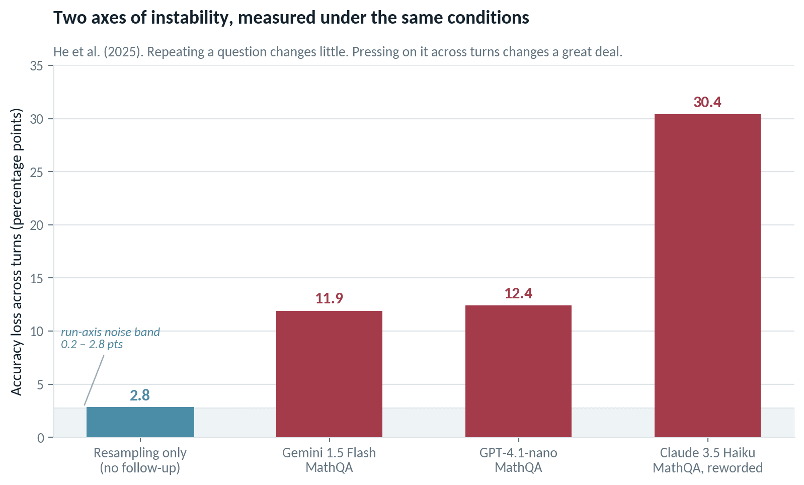
It does not. On MathQA, Gemini 1.5 Flash fell from 41.0 to 29.1 percent under the harshest follow-up, and GPT-4.1-nano from 31.5 to 19.1 percent. Claude 3.5 Haiku, tested with semantically equivalent reworded variants, dropped from 80.4 to 50.0 percent.
The control is what makes this usable. They re-ran 500 MathQA questions nine times each with no follow-up at all, which is pure resampling. Accuracy moved by 0.2 to 2.8 percent.
That is the cleanest available separation of the two axes. The turn axis carries several times the movement of the run axis, and current tooling still mostly ignores it.
3. Modelling a conversation as a Markov chain
The modelling contribution is why this paper matters outside its own field.
Rather than scoring each turn independently, treat the conversation as a system occupying one of two states and moving between them. The authors define state 1 as correct and state 0 as incorrect, then count four things across a training split: stays correct, correct to incorrect, incorrect to correct, and stays incorrect. Two probabilities fall out, p_TF (correct to incorrect) and p_FT (incorrect to correct), which form a transition matrix. Apply it repeatedly to the starting accuracy and you get a simulated trajectory.
They validated on a held-out 20 percent. Turn-10 deviation between simulated and observed accuracy was 0.38 percent for GPT-4.1-nano and 3.76 percent for Gemini 1.5 Flash on MathQA, with log loss and MSE reported per prompt type. The chain is a fitted model that predicts held-out behaviour, not a metaphor.
A two-state chain with non-zero transition probabilities converges. Run it forward and it settles at a stationary accuracy:
Acc(∞) = p_FT / (p_TF + p_FT)
The important thing about that expression is what is missing from it. The starting accuracy does not appear. Where the system ends up is a function of the transition rates alone. Across their configurations, Gemini 1.5 Flash landed roughly 8 to 12 percent below its first-turn accuracy on average, and Claude 3.5 Haiku on MathQA lost 34.82 points of stationary accuracy under the harshest reworded prompt.
4. What this looks like for a brand
Redefine the two states and nothing else about the machinery changes.
- State 1 (In): the brand appears in the recommendation set at this turn.
- State 0 (Out): it does not.
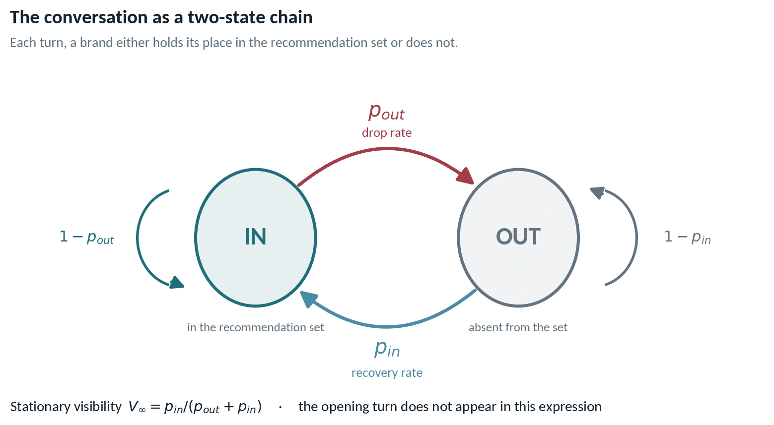
Renaming the transition probabilities gives a content team something to act on.
| Formal | GEO reading | Definition |
|---|---|---|
| p_TF | Drop rate (p_out) | P(brand absent at turn n+1 given present at turn n) |
| p_FT | Recovery rate (p_in) | P(brand present at turn n+1 given absent at turn n) |
| Acc(∞) | Stationary visibility (V∞) | Long-run probability of presence at an arbitrary deep turn |
Table 2. Translating the formal parameters into operational ones.
V∞ = p_in / (p_out + p_in)
Writing ρ = p_in / p_out turns this into V∞ = ρ / (1 + ρ). Stationary visibility depends on one thing: how much better you are at coming back than at falling out. Your opening position is not in the equation.
This is the formal reason first-response visibility fails to predict final recommendation. The two are an initial condition and a fixed point of a dynamical system, which are mathematically independent objects. Asking your discovery score to predict your decision-turn outcome is a category error rather than a measurement shortfall you can close with more samples.
5. Which three numbers matter
The transition matrix has a second eigenvalue, λ₂ = 1 − p_out − p_in, which governs how fast the system forgets where it started. Deviation from stationary shrinks geometrically, and the visibility half-life is:
n₁/₂ = ln(0.5) / ln|λ₂|
| Parameter | Question it answers | Where to intervene |
|---|---|---|
| p_out, drop rate | How fragile is the position once held? | Evidence and honest boundaries for the specific objection driving exits |
| p_in, recovery rate | Can the brand re-enter after being dropped? | Corpus coverage on the axes competitors currently own |
| n₁/₂, half-life | How long does the opening position last? | Structural. This decides whether first-response monitoring deserves budget |
Table 3. Three parameters, three separable diagnoses.
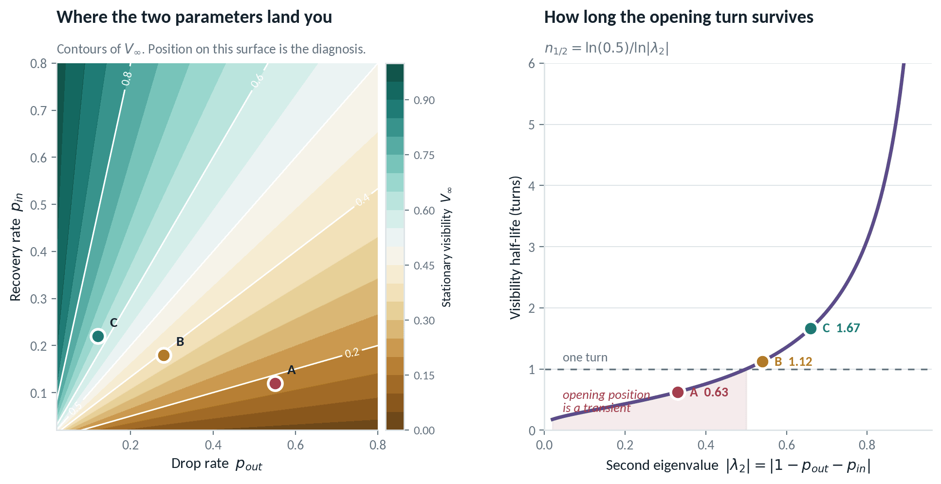
The left panel repays attention. Every brand in your category occupies a point on that surface, and its position is the diagnosis. Moving left is a survival problem. Moving up is a coverage problem. The contours are straight lines through the origin, so only the ratio of the two rates decides where you land, while their sum decides how fast you get there.
Half-life is the parameter most teams need first and rarely compute. It tells you whether your dashboard measures something durable or something the system discards before the buyer's second message.
6. What mention persistence actually measures
Persistence is the metric most likely to appear on a conversation analytics dashboard, and it is also the one most likely to be ambiguous. The chain makes the ambiguity precise, because two different quantities both deserve the name.
Spell persistence is the mean length of an uninterrupted run in the set. Once present, the brand survives each turn with probability 1 − p_out, so run length is geometric: E[spell] = 1 / p_out.
Total presence is the expected number of turns present across a ladder of length N, which is the sum of the trajectory. These two diverge whenever p_in is non-trivial, meaning whenever brands get dropped and picked back up, which is the normal case.
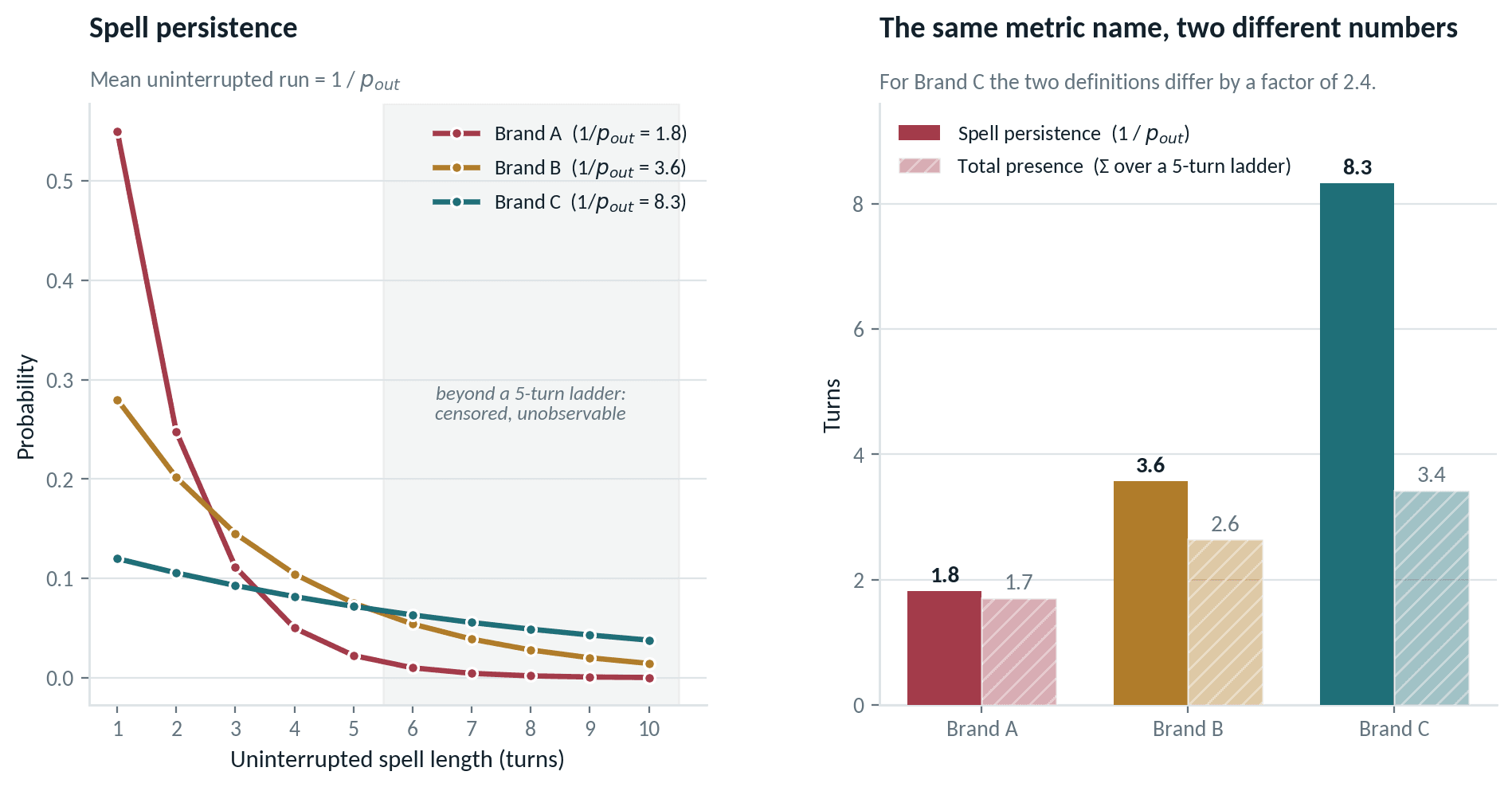
For the three brands below, spell persistence reads 1.8, 3.6 and 8.3 turns while total presence over a five-turn ladder reads 1.7, 2.6 and 3.4. Brand A's two figures nearly agree. Brand C's differ by a factor of 2.4. A vendor reporting "mention persistence: 3.4 turns" has told you almost nothing until they say which calculation produced it.
The shaded region in the left panel is a live methodological risk rather than a theoretical one. Spell persistence is censored by ladder length. On a five-turn ladder, any spell that would have run six or nine or twelve turns is recorded as five. Brand C's true p_out of 0.12 implies a mean run of 8.3 turns, of which a five-turn ladder can observe at most 60 percent. A short ladder therefore cannot distinguish a very durable brand from a moderately durable one, and any persistence number computed from truncated spells is biased downward for exactly the brands performing best. Either report total presence, which is well defined for a fixed ladder, or estimate p_out directly from the transition counts and derive persistence from it, rather than averaging observed run lengths.
7. A worked example: three brands, one opening position
Take three brands a monitoring tool would report as identical. All three appear in 72 percent of first responses for the same category prompt. Fit a chain to each and they separate immediately.
By the fifth turn, a modest length for a real buying conversation, Brand A is present in roughly one conversation in five and Brand C in two out of three. A dashboard reporting 72 percent for all three is reporting a quantity the system discarded at the second turn.
| Brand | p_out | p_in | V∞ | λ₂ | Half-life | Spell persistence |
|---|---|---|---|---|---|---|
| A | 0.55 | 0.12 | 0.18 | 0.33 | 0.63 turns | 1.8 turns |
| B | 0.28 | 0.18 | 0.39 | 0.54 | 1.13 turns | 3.6 turns |
| C | 0.12 | 0.22 | 0.65 | 0.66 | 1.67 turns | 8.3 turns |
Table 4. Illustrative parameters chosen to span a plausible range. The method is the point, not these values.
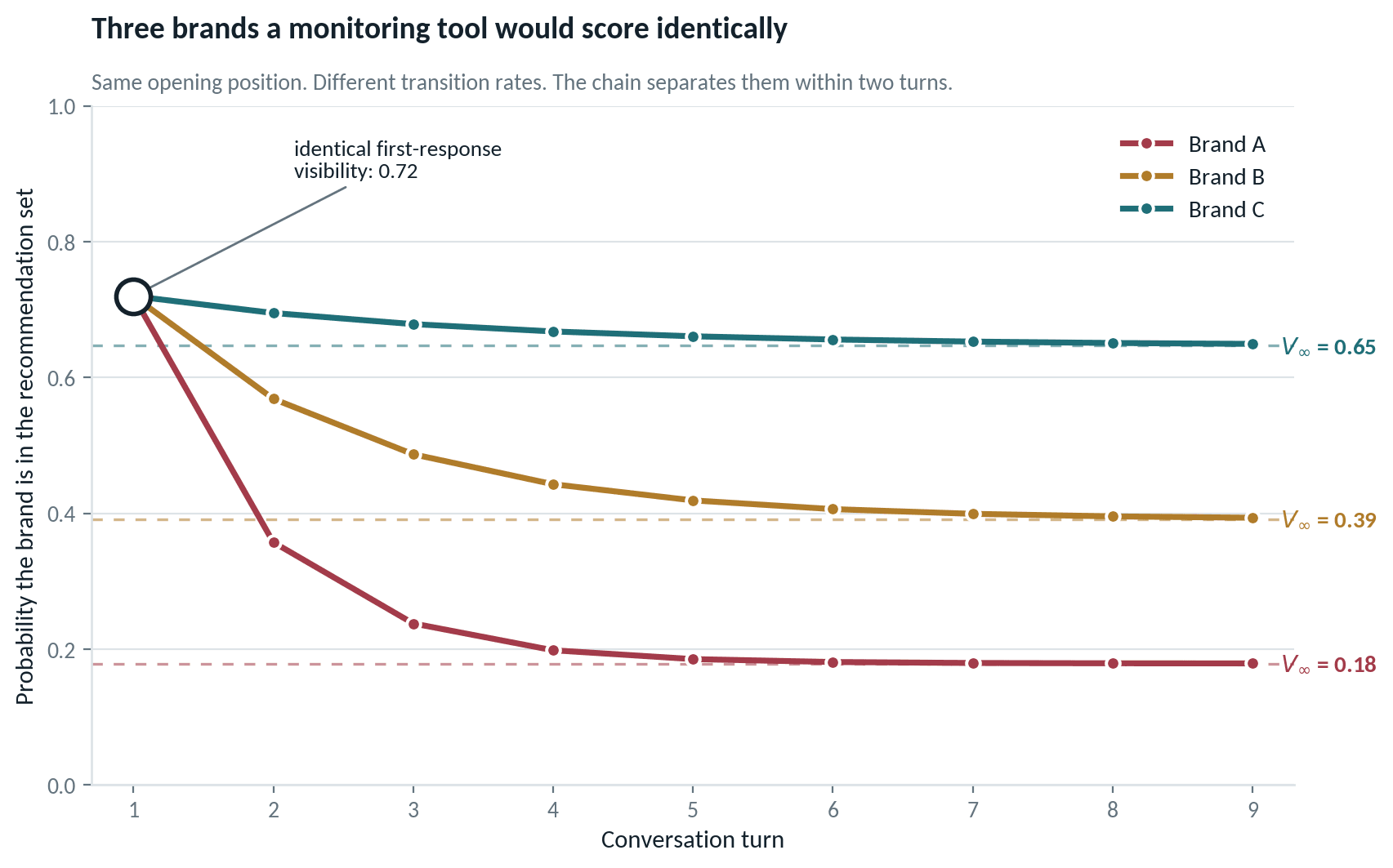
Brand A's half-life of 0.63 turns is the finding in that table. Its chain is essentially at equilibrium before the buyer's second message lands. There is no gradual erosion to intercept and no window in which the opening advantage is still worth defending. The 72 percent was a transient rather than a lead being lost.
8. When drift works in your favour
On Humanity's Last Exam, where GPT-4.1-nano starts at roughly 10 percent accuracy, multi-turn prompting pushed accuracy up by about two points. The Markov explanation is immediate: when you start below stationary, convergence moves you toward it. The chain reverts rather than rewarding or punishing.
Transposed to brand presence, multi-turn conversation compresses the gap between the discovery leader and everyone below it. Whoever sits above their stationary visibility loses ground, and whoever sits below it gains.
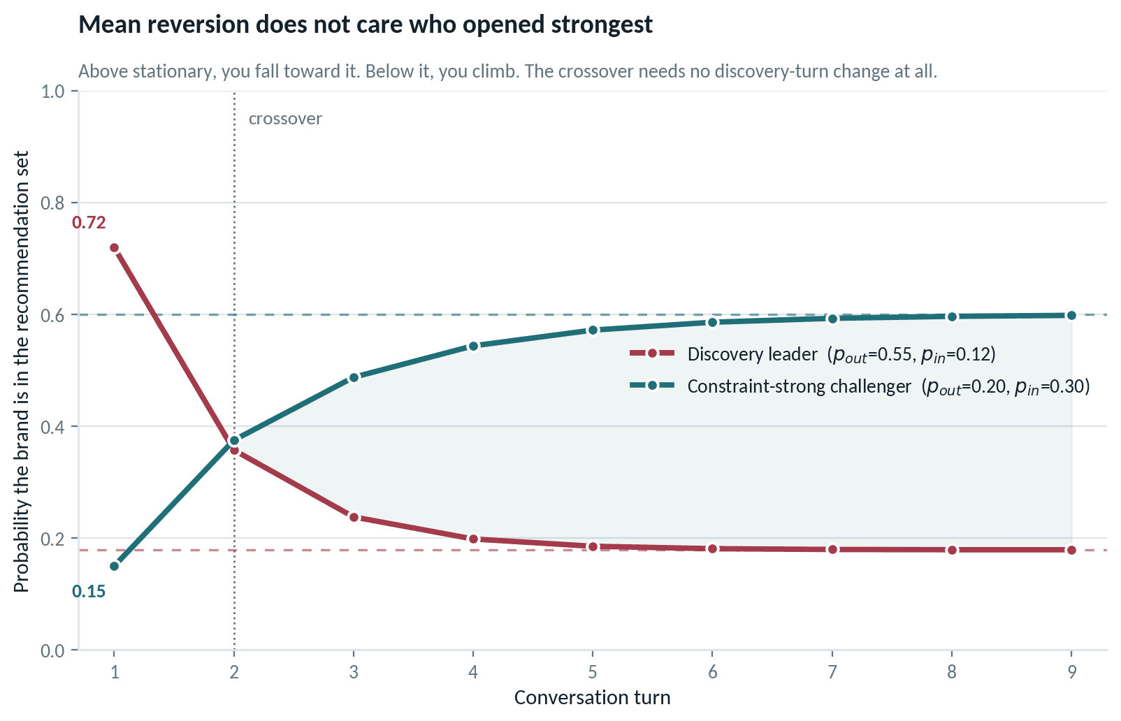
The challenger in that chart never improves its discovery-turn performance. It opens at 15 percent, a level most monitoring dashboards would treat as absent from the category, and holds majority presence from turn three onward purely because its transition rates are better.
If you have wondered why a competitor with a thin content footprint keeps appearing in your customers' AI-assisted shortlists, this is a hypothesis you can test rather than resent.
He et al.'s own caveat travels intact. Across their datasets, declines from above-stationary starts were substantially larger than the HLE gain. Reversion is not symmetric charity, and incumbents lose more than challengers gain.
9. Implications for the position-one playbook
C-SEO Bench delivered the strongest known single lever in this field. In their retail measurement, moving a source into context position one outperformed the best dedicated conversational SEO method by roughly 7.6 times. Retrieval position beats content tactics by a wide margin.
Set that next to the half-life result and a tension appears. Retrieval position acts most forcefully on the opening turn, and the opening turn is precisely the one whose influence decays fastest. For a brand with a high drop rate, it decays almost completely within one exchange.
This does not make position-one work useless, but it reframes what the work buys. Retrieval position sets a(1). It does not obviously touch p_out or p_in. In chain terms you are optimising the initial condition of a system that converges to a fixed point determined by other parameters.
Whether that is worth the investment depends on a number you can now compute. If your half-life is two turns and your conversations run four, initial position propagates meaningfully into the decision. If it is half a turn, you are paying for a transient. C-SEO Bench's second finding compounds this, since early-adopter advantages on their tested methods decay toward zero as adoption spreads. Initial-condition advantages are competitive and erodible. Transition-rate advantages, such as being the brand that survives a security question, are structural, and they rest on evidence a competitor has to produce rather than a tactic they can copy.
10. Where the model breaks
Three places, and skipping them would make this an advertisement rather than a method.
The mechanism is different. He et al. are substantially measuring sycophancy and pressure sensitivity, where a model abandons a correct answer because a user expressed doubt with no new evidence supplied. Brand drop-out under a genuine buyer constraint, such as a SOC 2 requirement, is closer to re-ranking on newly specified criteria. The mathematics transfers but the causal story does not, and the distinction is practical. Re-ranking is winnable with better evidence, and capitulation is not.
Memorylessness is an assumption with direct evidence against it. A first-order chain says turn n+1 depends only on turn n. Laban et al.'s central finding is that models which go wrong early tend not to recover, which in this vocabulary describes a near-absorbing state and a p_in that collapses after repeated exits rather than staying constant.
Time-homogeneity fails by construction on designed ladders. A standard chain uses one matrix for every step, but a constraint turn is deliberately built to have a higher p_out than a "tell me more" turn. Fitting one matrix across a designed ladder averages away the stage you were trying to isolate.
Each of those is testable, which is the subject of the next section.
11. The experiments
Already in the literature
These four are done, so cite them rather than repeating them.
| # | Experiment | Design and result | What it licenses |
|---|---|---|---|
| P1 | No-follow-up control (He et al.) | 500 MathQA questions repeated nine times with no follow-up prompt. Accuracy moved 0.2 to 2.8 percent | The null separating run-axis noise from turn-axis drift. Without it, observed drift is a resampling artefact |
| P2 | Simultaneous re-run (Schulte et al.) | Same prompt issued up to ten times within 24 hours, four engines, 3,409 pairwise comparisons. Brand Jaccard 0.33 to 0.48 | Instability is intrinsic model stochasticity, not index refresh |
| P3 | Sharded single vs multi-turn (Laban et al.) | One instruction delivered whole, then split across turns, over 200,000 simulated conversations. 39 percent average drop | Multi-turn is a distinct regime and exits may be near-absorbing |
| P4 | Multi-actor adoption sweep (Puerto et al.) | Nine C-SEO methods, six domains, 1,921 queries, sweeping adoption fraction. Early-adopter gain approaches zero at full adoption | Initial-condition advantages are competitive and erodible |
Table 5. Published experiments this argument rests on.
Still to run
Each is specified so a team can execute it this quarter.
E1. The constraint control. Build one five-turn ladder in two arms sharing an identical discovery turn. The constraint arm introduces real purchase criteria at turns 2 to 4, such as a price ceiling, compliance requirement, delivery window, or integration need. The neutral arm uses content-free follow-ups: "tell me more", "anything else?", "are you sure?". Run both across at least 40 replays per seed and at least 8 seeds, with one engine held fixed. Readout: churn in the final recommendation set per arm. Interpretation: if constraint-arm churn substantially exceeds neutral-arm churn, you are observing re-ranking on stated criteria and content investment is the right response. If the arms are comparable, you are observing pressure sensitivity, the model is wobbling rather than re-ranking, and no amount of evidence content will fix it. This must run before any fitted chain is acted on.
E2. Transition fit with held-out validation. Label every turn of every replay as present or absent per brand. Count the four transitions on 80 percent of conversations, fit p_out and p_in, then simulate forward from the held-out 20 percent and score against observed with log loss and MSE. Readout: per-turn deviation between simulated and observed visibility. Interpretation: deviation comparable to the paper's 0.4 to 3.8 percent means the chain holds on your data. Report effective sample size per parameter separately, since p_out is estimable only from turns where the brand was present and p_in only from turns where it was absent.
E3. Per-stage homogeneity test. Fit one transition matrix per ladder stage rather than one pooled matrix, and compare with a likelihood-ratio test. Readout: which stage carries the highest p_out. Interpretation: that stage is the diagnosis, and the pooled matrix is what hides it.
E4. Constraint inversion. Hold the discovery turn fixed and vary only the emphasised criterion across arms: lowest price, fastest delivery, strongest compliance, widest integration coverage. Readout: the winning brand per axis, and each brand's p_out per axis. Interpretation: if one brand wins under every axis, the model has a fixed favourite and constraint framing is not doing the work. If the winner changes with the axis, re-ranking is confirmed and each brand's per-axis drop rate names the objection costing it the deal.
E5. Order test. Fit a first-order chain, then a second-order model conditioning on whether the brand has already been dropped earlier in the conversation, and compare held-out log loss. Readout: whether p_in after two prior exits differs from p_in after one. Interpretation: this tests Laban et al.'s finding in the brand setting. If re-entry probability collapses with exit history, the state is near-absorbing and the simple V∞ formula overstates your recovery.
E6. Ladder-length censoring check. Run the same seeds on a five-turn and a ten-turn ladder and compute spell persistence both ways. Readout: the gap between estimates per brand. Interpretation: a large gap concentrated in your most durable brands confirms the censoring bias, and means persistence must be derived from p_out rather than averaged from observed runs.
Sequencing. E1 gates everything. E2 validates the model. E3 and E4 produce the content brief. E5 and E6 determine how much to trust the numbers E2 gives you. A team with one engine, eight seeds and forty replays can complete E1 through E4 from a single collection run, because all four read from the same labelled transcripts.
12. What changes in practice
- Report stationary visibility alongside first-response visibility. They are different quantities and one does not stand in for the other.
- Compute your half-life before deciding what first-turn monitoring is worth. A sub-one-turn half-life is a budget conclusion rather than a metrics footnote.
- Say which persistence you mean. Spell persistence and total presence answer different questions and can differ by more than a factor of two on the same brand.
- Diagnose by parameter. High
p_outis a survival problem calling for evidence against the objection that removes you. Lowp_inis a coverage problem, meaning you are not retrievable where a competitor is winning. - Fit separate matrices per constraint type. The variation between them names the buyer condition costing you, which is more actionable than "publish more".
- Read a strong opening as a liability when your drop rate is high. Mean reversion is indifferent to how good your discovery number looked.
- Keep the resampling discipline. Nothing here replaces repeated measurement. You need enough runs to estimate each turn's rate and enough turns to estimate the transitions between them, and forty replays of a five-turn ladder gives you both from one collection.
AI visibility measurement solved its first statistical problem, the unreliability of single observations, with real rigour, and then stopped. The second problem is a directional process with a fixed point. It has been formally modelled and validated on held-out data in an adjacent literature, and the fitting procedure is four counts and a division.
To measure multi-turn visibility and transition rates on your own category prompts, see Analytika.
References
- Aggarwal, P., Murahari, V., Rajpurohit, T., Kalyan, A., Narasimhan, K., & Deshpande, A. (2024). GEO: Generative Engine Optimization. KDD 2024. arXiv:2311.09735
- He, J., Ramachandran, R., Ramachandran, N., Katakam, A., Zhu, K., Dev, S., Panda, A., & Shrivastava, A. (2025). Modeling and Predicting Multi-Turn Answer Instability in Large Language Models. NeurIPS 2025 Workshop on Multi-Turn Interactions in LLMs. arXiv:2511.10688
- Laban, P., Hayashi, H., Zhou, Y., & Neville, J. (2025). LLMs Get Lost In Multi-Turn Conversation. arXiv:2505.06120
- Puerto, H., Gubri, M., Green, T., Oh, S. J., & Yun, S. (2025). C-SEO Bench: Does Conversational SEO Work? NeurIPS 2025 Datasets & Benchmarks Track. arXiv:2506.11097
- Schulte, J., Bleeker, M., & Kaufmann, P. (2026). Don't Measure Once: Measuring Visibility in AI Search (GEO). arXiv:2604.07585
Vignesh Kanike is Founding Engineer at AEOsim, working on measurement methods for multi-turn AI visibility. This piece was originally published on The GEO Community. For the product framing of multi-turn survival across the buying conversation, see Conversation Analytics: Chat Is the New Funnel. On how alternative clarifying answers move the recommendation set beyond run-to-run noise, see Clarification as a Branch Point. Run the multi-turn measurement layer with Analytika.